Lab 9.2 – Using Excel References with Workbook Part 2
Configure Named Ranges
Step 22. In the workbook, click the Sheet2 worksheet.
Step 23. Click Tag Selection, and then click Tag Selection.
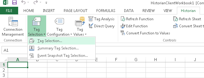
The Tag Selection dialog box appears.
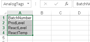
Step 24. Select the following tags:
- BatchNumber
- ProdLevel
- ReactLevel
- ReactTemp
Step 25. Ensure that the value for the Selected cell range to insert tags is $A$1.
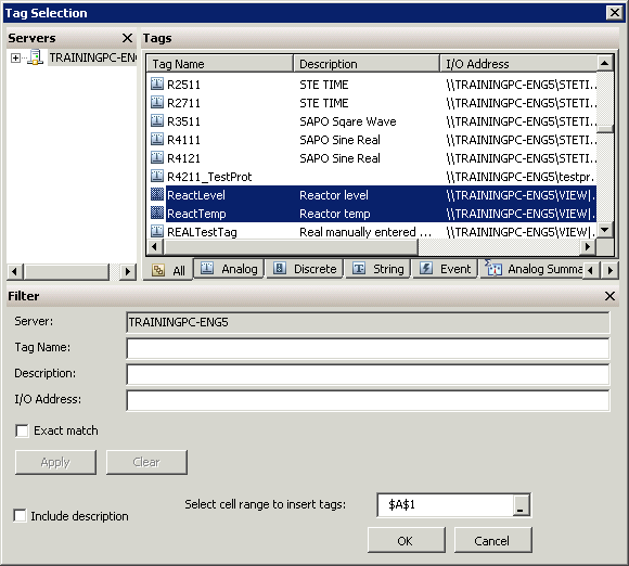
Step 26. Click OK.
Step 27. Select cells A1 through A4.
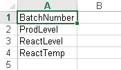
Step 28. In the name box, enter AnalogTags and press Enter.
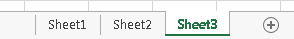
Step 29. In the workbook, click the Sheet3 worksheet.
Placing the named range tag list to another sheet in the workbook enables better formatting with less duplication of tag names.
Step 30. Click cell A1.
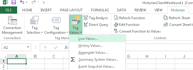
Step 31. Click Tag Values, and then click Live Values.
The Live Values - Step 1 of 3 dialog box appears.
Step 32. In the Select cell(s) containing tag name(s) field, enter AnalogTags.
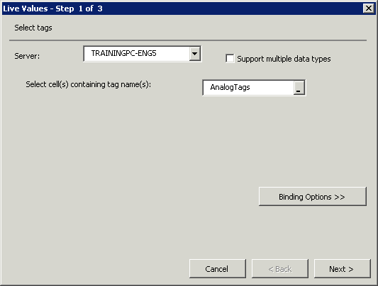
Step 33. Click Next.
The Live Values - Step 2 of 3 dialog box appears.
Step 34. In the Select cell for output field, click in the middle of the field and then click cell A1. Ensure that the cell reference is Sheet3!$A$1.
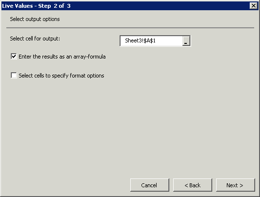
Step 35. Click Next.
The Live Values - Step 3 of 3 dialog box appears.
Step 36. Retain the default values.
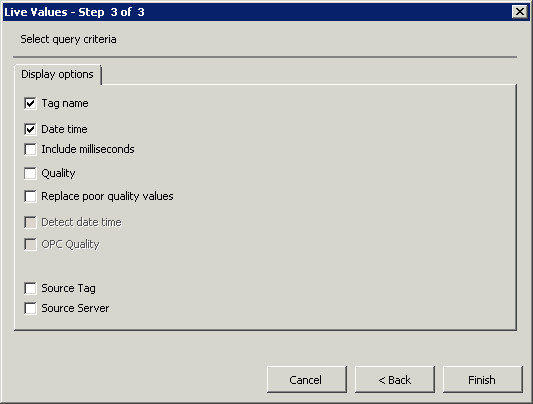
Step 37. Click Finish.
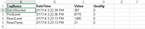
The tag name range is inserted into the worksheet.
Step 38. In the workbook, click the Sheet2 worksheet.
Step 39. Replace the BatchNumber tag with M100.LT.PV tag.
Step 40. Replace the ProdLevel tag with Inlet1_001.PV tag.
Step 41. Replace the ReactLevel tag with Outlet_001.PV tag.
Step 42. Replace the ReactTemp tag with M100.TT.PV tag.
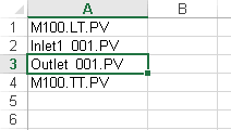
Step 43. On the workbook, click the Sheet3 worksheet to observe the changes.
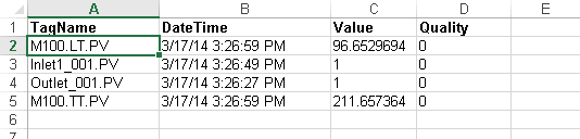
Save the report as Configure Named Ranges.xlsx in the C:\Training folder and close the
Last modified: Wednesday, 13 May 2020, 7:54 PM