Insert an Aggregate Value Function

Step 1. Create a new workbook with three blank worksheets.

Step 2. Select Sheet1.

Step 3. In cell A1, enter SysTimeSec and press Enter.

Step 4. In cell A3, enter Start Time and press Enter.

Step 5. In cell A4, enter End Time and press Enter.

Step 6. Expand Column A as desired.

Step 7. In cell B3, enter a date and time relative to class time as the Start Time value and press Enter.

Step 8. In cell B4, enter a date and time 5 minutes later than the Start Time value specified in step 5 as the End Time value and press Enter.

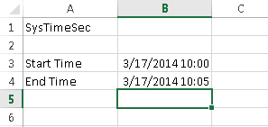
The workbook should now appear as follows:

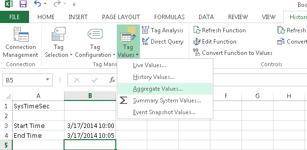
Step 9. On the Historian menu ribbon, click Tag Values, and then click Aggregate Values.

The Aggregate Values - Step 1 of 4 dialog box appears.

Step 10. In the Select cell(s) containing tag name(s) field, click in the middle of the field, and then select cell A1. Ensure that the field’s cell reference is Sheet1!$A$1.

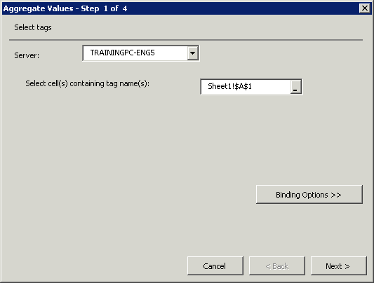
Step 11. Click Next.

The Aggregate Values - Step 2 of 4 dialog box appears.

Step 12. In the Select cell for output field, click in the middle of the field, and then select cell A7. Ensure that the field’s cell reference is Sheet1!$A$7 and that the Enter the results as an array-formula check box is checked.

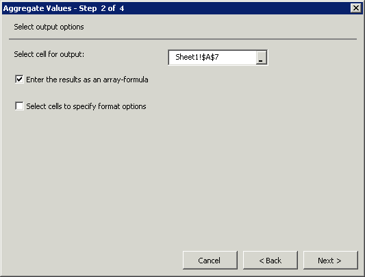
Step 13. Click Next.

The Aggregate Values - Step 3 of 4 dialog box appears. 

Step 14. Click the Calculations tab.

Step 15. In the Calculation type drop-down list, click Average.

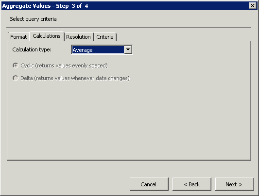
Step 16. Click Next.

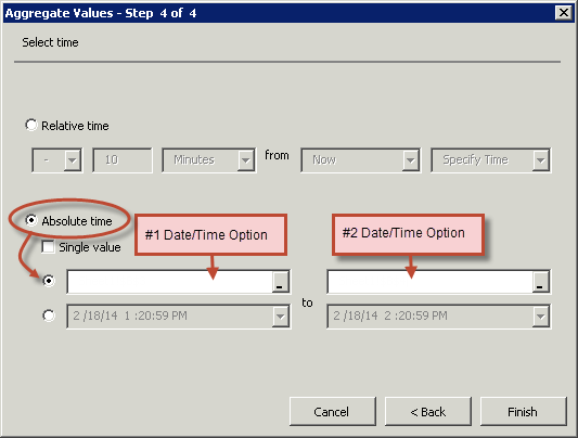
The Aggregate Values - Step 4 of 4 dialog box appears.

Step 17. Click the Absolute time option.

Step 18. Under the Absolute time option, click the first date and time option.

Step 19. In the field on the left, specify the cell reference as Sheet1!$B$3. 

Step 20. In the field on the right, specify the cell reference as Sheet1!$B$4.

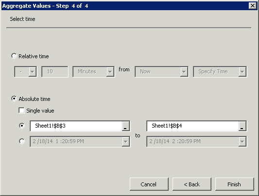
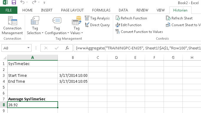
Step 21. Click Finish.

The aggregate value appears in the worksheet.